Introduction

Info

Please cite this library by citing the corresponding paper or Zenodo reference XXX “”.

About PyXC

PyXC is a point-to-point correlation tool based on Python. This library aims for a self-documenting correlation library on top of the IPython environment.

Purpose of this tool

This library was initially developed for a correlation task between nano-indentation and EBSD measurements. The main targets of this tool are:

• To provide a self-explaining correlation library based on the Jupyter Notebook environment.

• To provide a flexible environment for correlation between 2-dimensionally sampled data.

Common workflow

To perform a correlation, several crucial steps are required to be cleared out. Correlation steps can be divided into four different parts. Each step is dealt with in a respective tutorial notebook.

1. Parsing data from the data file.

2. Loading data into the library.

3. Correcting distortion between different measurements.

4. Make a correlation.

Usage

This library is able to perform a coordinate-based correlation task which enables the correlation between different scientific data sets.

# Load EBSD data
import numpy as np

EBSD = np.genfromtxt(
    "./data/SiC_in_NiSA.ctf", dtype=float, skip_header=15, delimiter="\t", names=True
)

# Load data into the layer
from pyxc.core.layer import Layer
from pyxc.core.processor.arrays import column_parser
from pyxc.core.container import Container2D
from pyxc.core.loader import ImageLoader, XYDLoader
from pyxc.transform.homography import Homography

layer_ebsd = Layer(
    data=column_parser(EBSD, format_string="dxydddddddd"),
    container=Container2D,
    dataloader=XYDLoader,
    transformer=Homography,
)

It can query the datapoints based on the given (x, y) coordinates.

layer_ebsd.query(
    3,
    3,
    cutoff=2,
    output_number=5,
)

array([(1111, 3.0541, 3.0541, 3.0541, 3.0541, 2., 10., 0., 160.98, 48.262, 233.64, 1.2168, 175., 255., 0, 0.07650901, 3, 3),
       (1110, 2.7765, 3.0541, 2.7765, 3.0541, 2., 11., 0., 160.16, 48.818, 234.65, 1.3001, 160., 255., 0, 0.2299545 , 3, 3),
       (1011, 3.0541, 2.7765, 3.0541, 2.7765, 2., 10., 0., 160.6 , 48.47 , 233.71, 1.1951, 162., 255., 0, 0.2299545 , 3, 3),
       (1010, 2.7765, 2.7765, 2.7765, 2.7765, 2., 11., 0., 160.49, 48.59 , 233.56, 1.2747, 159., 255., 0, 0.31607675, 3, 3),
       (1211, 3.0541, 3.3318, 3.0541, 3.3318, 2., 11., 0., 160.6 , 48.849, 234.49, 1.3554, 168., 255., 0, 0.33618156, 3, 3)],
      dtype=[('row', '<u2'), ('x', '<f4'), ('y', '<f4'), ('x_raw', '<f4'), ('y_raw', '<f4'), ('Phase', '<f8'), ('Bands', '<f8'), ('Error', '<f8'), ('Euler1', '<f8'), ('Euler2', '<f8'), ('Euler3', '<f8'), ('MAD', '<f8'), ('BC', '<f8'), ('BS', '<f8'), ('query_index', '<i8'), ('distance', '<f8'), ('x-coordinates', '<i8'), ('y-coordinates', '<i8')])

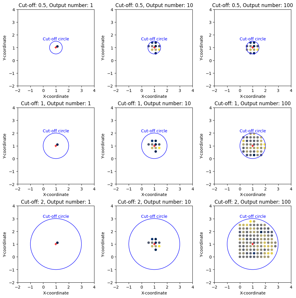
Query operation is based on the given (x, y) coordinates. The cutoff parameter is used to determine the maximum distance between the given (x, y) coordinates and the queried data points. The output_number parameter is used to determine the maximum number of data points to be returned.

import matplotlib.pyplot as plt

xy = (1, 1)
cutoff = [0.5, 1, 2]
output_number = [1, 10, 100]
fig, ax = plt.subplots(3, 3, figsize=(10, 10), constrained_layout=True)

for i, c in enumerate(cutoff):
    for j, o in enumerate(output_number):
        qr = layer_ebsd.query(*xy, cutoff=c, output_number=o)
        ax[i, j].scatter(qr["x"], qr["y"], c=qr["BC"], s=25, cmap="cividis")
        ax[i, j].set_title(f"Cut-off: {c}, Output number: {o}")
        ax[i, j].set_aspect(1)

        ax[i, j].scatter(*xy, marker="+", color="Red")

        ax[i, j].add_patch(
            plt.Circle(xy, radius=c, edgecolor="Blue", facecolor=[0, 0, 0, 0])
        )
        ax[i, j].annotate(
            "Cut-off circle", (xy[0], xy[1] + c), color="Blue", ha="center", va="bottom"
        )
        ax[i, j].set_xlabel("X-coordinate")
        ax[i, j].set_ylabel("Y-coordinate")
        ax[i, j].set_aspect(1)

        ax[i, j].set_xlim(-np.max(cutoff) * 1.5 + xy[0], np.max(cutoff) * 1.5 + xy[0])
        ax[i, j].set_ylim(-np.max(cutoff) * 1.5 + xy[1], np.max(cutoff) * 1.5 + xy[1])

You can use Reducer to reduce the number of data points to be returned. Especially good for the statistical analysis of the data.

from pyxc.core.processor.reducer import Reducer
import numpy as np

layer_ebsd.query(3, 3, cutoff=5, output_number=1000, reducer=Reducer((np.mean,)))

array([(760, 0, 3., 3., 3.64924645, 3.64924645, 1327, 3.6492465, 3.6492465, 3.6492465, 3.6492465, 2., 10.06973684, 0., 160.42452632, 48.3094, 233.93259211, 1.14091868, 163.11052632, 255., 0, 3.00931105, 3, 3)],
      dtype=[('count', '<i8'), ('query_index', '<i8'), ('x-coordinates', '<f8'), ('y-coordinates', '<f8'), ('avg_x', '<f8'), ('avg_y', '<f8'), ('row_mean', '<u2'), ('x_mean', '<f4'), ('y_mean', '<f4'), ('x_raw_mean', '<f4'), ('y_raw_mean', '<f4'), ('Phase_mean', '<f8'), ('Bands_mean', '<f8'), ('Error_mean', '<f8'), ('Euler1_mean', '<f8'), ('Euler2_mean', '<f8'), ('Euler3_mean', '<f8'), ('MAD_mean', '<f8'), ('BC_mean', '<f8'), ('BS_mean', '<f8'), ('query_index_mean', '<i8'), ('distance_mean', '<f8'), ('x-coordinates_mean', '<i8'), ('y-coordinates_mean', '<i8')])