Tutorial 1. Quick Tutorial

General process

The process of correlation is composed of five steps:

1. Loading data

2. Processing data

3. Loading data into a layer object

4. Fixing distortion

5. Performing the correlation

In this tutorial, we’ll guide you through these steps with focus on a particular type of data: an EBSD mapping result of a plastic deformation field around a carbide particle in a nickel-based superalloy.

Loading Data

Loading data is an essential first step in the correlation process. The type of data to be loaded can vary greatly depending on the specific context or project you are working on. Here, we’ll demonstrate how to load an example EBSD (Electron Backscatter Diffraction) file.

In this case, we’re going to use the genfromtxt method from the NumPy library to load the data into a structured array. Once loaded, we can visually examine the data by plotting it using matplotlib.

# Load EBSD data
import numpy as np

EBSD = np.genfromtxt(
    "./data/SiC_in_NiSA.ctf", dtype=float, skip_header=15, delimiter="\t", names=True
)

Upon successful loading, the data can be examined. It is crucial to understand the nature of the data, its structure and its attributes, as these factors could significantly affect the subsequent steps in the process.

# Check EBSD data
import matplotlib.pyplot as plt

fig, axs = plt.subplots(1, 2, constrained_layout=True)

axs[0].scatter(EBSD["X"], EBSD["Y"], c=EBSD["BC"], s=2, cmap="gray")
axs[0].set_title("BC")

axs[1].scatter(EBSD["X"], EBSD["Y"], c=EBSD["Phase"], s=2, cmap="cividis", vmax=4)
axs[1].set_title("Phase")

for ax in axs:
    ax.set_aspect(1)

Let’s examine the resulting structured array.

EBSD

array([(2.,  0.    ,  0.   , 11., 0., 160.45, 47.733, 233.82, 1.0211, 160., 255.),
       (2.,  0.2776,  0.   , 10., 0., 160.15, 47.888, 233.74, 1.3246, 161., 255.),
       (2.,  0.5553,  0.   , 10., 0., 160.14, 47.928, 234.  , 1.3319, 161., 255.),
       ...,
       (2., 26.932 , 20.546, 11., 0., 159.7 , 48.268, 235.35, 1.2136, 154., 255.),
       (2., 27.21  , 20.546, 10., 0., 159.24, 48.137, 234.97, 0.861 , 159., 255.),
       (2., 27.487 , 20.546, 10., 0., 158.98, 48.32 , 235.21, 1.125 , 162., 255.)],
      dtype=[('Phase', '<f8'), ('X', '<f8'), ('Y', '<f8'), ('Bands', '<f8'), ('Error', '<f8'), ('Euler1', '<f8'), ('Euler2', '<f8'), ('Euler3', '<f8'), ('MAD', '<f8'), ('BC', '<f8'), ('BS', '<f8')])

Loading Data Into the Layer

The Layer object represents a layer of measurement for a material, such as EBSD data. In this tutorial, we are going to discuss how to load EBSD data into a Layer object. More comprehensive details about constructing and manipulating a Layer object will be covered in later tutorials.

Direct construction of the Layer object

We can create a Layer object and load our data into it directly. Here is a example:

# Load data into the layer
from pyxc.core.layer import Layer
from pyxc.core.processor.arrays import column_parser
from pyxc.core.container import Container2D
from pyxc.core.loader import ImageLoader, XYDLoader
from pyxc.transform.homography import Homography

layer_ebsd = Layer(
    data=column_parser(EBSD, format_string="dxydddddddd"),
    container=Container2D,
    dataloader=XYDLoader,
    transformer=Homography,
)

Dealing with geometric distortions

Given that we’ve opted for the Homography transformation method, we’ll employ a 3x3 transformation matrix. This matrix can be constructed using various libraries, including OpenCV. For now, let’s proceed under the assumption that we already possess the necessary transformation matrix to rectify the distortions in our layer.

Don’t forget to explicitly apply the transformation.

# Apply transformation to the layer
transformation_matrix = np.array(
    [
        [1, 0.1, 10],
        [0, 1.0, 30],
        [0, 0.0, 1],
    ]
)

layer_ebsd.set_transformation_matrix(transformation_matrix)
layer_ebsd.apply_transformation()

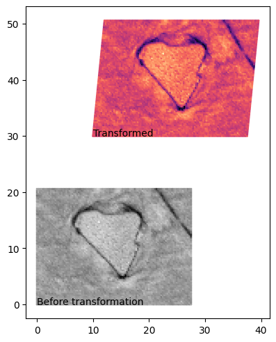
Let’s quickly check whether the transformation is correctly applied.

# Check EBSD data
import matplotlib.pyplot as plt

fig, ax = plt.subplots(constrained_layout=True)

ax.scatter(
    layer_ebsd.container["x_raw"],
    layer_ebsd.container["y_raw"],
    c=layer_ebsd.container["BC"],
    s=2,
    cmap="gray",
)
ax.text(0, 0, "Before transformation")

ax.scatter(
    layer_ebsd.container["x"],
    layer_ebsd.container["y"],
    c=layer_ebsd.container["BC"],
    s=2,
    cmap="magma",
)
ax.text(10, 30, "Transformed")

ax.set_aspect(1)

Querying by (X, Y) Coordinates

It is possible to retrieve data for a specific location by querying with (X, Y) coordinates. Two parameters, ‘cut-off’ and ‘output_number’, play crucial roles in this process.

The ‘cut-off’ parameter determines the maximum Euclidean distance from the query point \((X_{\text{query}}, Y_{\text{query}})\) to a nearby data point \((X_{\text{data}}, Y_{\text{data}})\) beyond which the data point will be disregarded.

The ‘output_number’ parameter specifies the maximum number of closest valid data points to the query point that will be returned. For instance, if there are 10 valid data points within the cut-off circle and ‘output_number’ is set to 5, only the nearest 5 points will be returned.

Let’s explore the query method. If no valid data points are found near the query point, a NaN (Not a Number) value will be returned.

# Query data (after transformation there is no point in 10, 10 coordinate
query_invalid = layer_ebsd.query(10, 10, cutoff=5, output_number=10)

query_invalid

/home/docs/checkouts/readthedocs.org/user_builds/pyxc/envs/latest/lib/python3.11/site-packages/pyxc/core/layer.py:317: UserWarning: Couldn't find the matching point. Please ignore rows containing NaN.
  warn("Couldn't find the matching point. Please ignore rows containing NaN.")

array([],
      dtype=[('row', '<i4'), ('x', '<f4'), ('y', '<f4'), ('x_raw', '<f4'), ('y_raw', '<f4'), ('Phase', '<f8'), ('Bands', '<f8'), ('Error', '<f8'), ('Euler1', '<f8'), ('Euler2', '<f8'), ('Euler3', '<f8'), ('MAD', '<f8'), ('BC', '<f8'), ('BS', '<f8'), ('query_index', '<i8'), ('distance', '<f8'), ('x-coordinates', '<f8'), ('y-coordinates', '<f8')])

In the case that valid data points exist within the ‘cut-off’ distance from the query point, the query method will successfully return the data corresponding to these points, up to the limit set by ‘output_number’.

query_valid = layer_ebsd.query(30, 40, cutoff=5, output_number=10)

query_valid

array([(3668, 29.87953 , 39.9953, 18.88 ,  9.9953, 2., 10., 0., 162.08, 47.098, 232.46, 0.9581, 161., 255., 0, 0.12056168, 30, 40),
       (3669, 30.157532, 39.9953, 19.158,  9.9953, 2., 10., 0., 161.24, 47.226, 232.96, 1.034 , 167., 255., 0, 0.15760183, 30, 40),
       (3768, 29.907299, 40.273 , 18.88 , 10.273 , 2.,  9., 0., 162.24, 47.187, 232.25, 0.947 , 158., 255., 0, 0.28830855, 30, 40),
       (3569, 30.12977 , 39.7177, 19.158,  9.7177, 2., 10., 0., 160.78, 47.189, 233.08, 1.0312, 164., 255., 0, 0.31069772, 30, 40),
       (3568, 29.851768, 39.7177, 18.88 ,  9.7177, 2., 10., 0., 161.7 , 46.981, 232.5 , 1.0163, 161., 255., 0, 0.31885001, 30, 40),
       (3769, 30.1853  , 40.273 , 19.158, 10.273 , 2., 10., 0., 161.02, 48.041, 233.02, 1.2996, 152., 255., 0, 0.32994658, 30, 40),
       (3667, 29.60153 , 39.9953, 18.602,  9.9953, 2., 10., 0., 162.74, 47.019, 232.24, 0.9985, 167., 255., 0, 0.39849764, 30, 40),
       (3670, 30.43453 , 39.9953, 19.435,  9.9953, 2.,  9., 0., 161.05, 47.463, 232.94, 0.9628, 164., 255., 0, 0.43455567, 30, 40),
       (3767, 29.6293  , 40.273 , 18.602, 10.273 , 2., 10., 0., 162.42, 47.313, 232.01, 0.9826, 162., 255., 0, 0.46037752, 30, 40),
       (3570, 30.406769, 39.7177, 19.435,  9.7177, 2., 10., 0., 160.78, 47.189, 233.08, 1.0312, 172., 255., 0, 0.49512989, 30, 40)],
      dtype=[('row', '<i4'), ('x', '<f4'), ('y', '<f4'), ('x_raw', '<f4'), ('y_raw', '<f4'), ('Phase', '<f8'), ('Bands', '<f8'), ('Error', '<f8'), ('Euler1', '<f8'), ('Euler2', '<f8'), ('Euler3', '<f8'), ('MAD', '<f8'), ('BC', '<f8'), ('BS', '<f8'), ('query_index', '<i8'), ('distance', '<f8'), ('x-coordinates', '<i8'), ('y-coordinates', '<i8')])

A Reducer object allows for the execution of statistical operations on your data. This capability is especially useful when you have multiple data points, i.e., when ‘output_number’ is more than 1.

The Reducer object’s format is defined as Iterable[Tuple[Callable, Iterable[Column Names]]]. In this structure, Callable refers to the statistical function to be applied, while Iterable[Column Names] is a list of the columns on which this function will be applied.

When you use a Reducer object, the resulting query columns will be altered. The new format of each column will be ColumnName_CallableName, where CallableName is the name of the statistical function applied and ColumnName is the original column name.

from pyxc.core.processor.reducer import Reducer

reducer_obj = Reducer([(np.mean, ["BS", "Phase"]), (np.std, ["BS", "Phase"])])
query_valid_with_reducer = layer_ebsd.query(
    30, 40, cutoff=5, output_number=10, reducer=reducer_obj
)

query_valid_with_reducer

array([(10, 0, 30., 40., 30.01833534, 39.99533081, 255., 2., 0., 0.)],
      dtype=[('count', '<i8'), ('query_index', '<i8'), ('x-coordinates', '<f8'), ('y-coordinates', '<f8'), ('avg_x', '<f8'), ('avg_y', '<f8'), ('Phase_mean', '<f8'), ('BS_mean', '<f8'), ('Phase_std', '<f8'), ('BS_std', '<f8')])

Also, when the ‘output_number’ is set to more than 1 (to use execute_query method), it becomes necessary to supply a Reducer object. This is because when multiple rows of data are returned by each query, there is ambiguity about how to consolidate these results into a single array. To resolve this, the Reducer object is employed to reduce these multiple rows of data into a single entry, thus ensuring a consistent data structure.

xs, ys = np.meshgrid(np.arange(20, 30, 1), np.arange(35, 45, 1))
xs, ys = xs.flatten(), ys.flatten()

bulk_query = layer_ebsd.execute_queries(
    xs, ys, cutoff=2, output_number=2, reducer=reducer_obj
)

Maximum worker:  6

Executing queries: 100%|██████████| 100/100 [00:00<00:00, 300882.64it/s]

In addition, it is feasible to perform multiple queries simultaneously for added convenience. These queries are executed in parallel to enhance efficiency.

Warning

See the code below very carefully. There is no guarantee that all points that you have provided yield a correlation result. If the points are too far away from the data point (beyond the cut-off distance), you will not get the result. You will be required to filter out the points that are not hit by using the query_index column.

xs, ys = np.meshgrid(np.arange(20, 30, 1), np.arange(35, 45, 1))
xs, ys = xs.flatten(), ys.flatten()

bulk_query = layer_ebsd.execute_queries(xs, ys, cutoff=2, output_number=1)

xs_filtered = xs[bulk_query["query_index"]]
ys_filtered = ys[bulk_query["query_index"]]

Maximum worker:  6

Executing queries: 100%|██████████| 100/100 [00:00<00:00, 156913.73it/s]

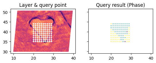
Let’s check the query result.

fig, ax = plt.subplots(1, 2, sharex="all", sharey="all")

ax[0].scatter(*layer_ebsd.get_xy(), c=layer_ebsd.container["BC"], cmap="magma", s=1)
ax[0].scatter(xs, ys, c="#ffffff", marker="+", s=20)
ax[0].set_title("Layer & query point")

ax[1].scatter(
    bulk_query["x-coordinates"], bulk_query["y-coordinates"], c=bulk_query["Phase"], s=1
)
ax[1].set_title("Query result (Phase)")

for a in ax:
    a.set_aspect(1)