Tutorial 2. Parsing a data

Info

This section is not really connected to this library. This section is prepared to demonstrate how to read scientific data. This section itself is not mandatorily required to proceed with a correlation task. However, often scientific data requires own parsers to read it. In that case, this section might help you.

Python libraries used in this section other than PyXC

• Pandas (pandas)

• Numpy (numpy)

• Scikit Image (scikit-image)

Parsing a data

This is intended for the basic course if you are not familiar with Python. If you can read your own data into a NumPy array or Python iterables, you can skip this tutorial.

One best case to read data is finding a library which is able to handle the format you want to read in. For example, the hyperspy module is able to read .spd files to build an integrated window map. Utilizing pre-written libraries drastically reduces the time for the correlation. If desired file readers are not available, it will be required to build a code snippet for that purpose.

This section explains about how to read scientific data if appropriate readers are not available. In most cases it is not an issue.

Rule of Thumb

1. Find the library that can read your data.

2. Export your data to easily readable formats.

3. Try to implement the reader if that is absolutely necessary

Common practice to reading data

Info: This section is prepared to demonstrate how to read scientific data. This section itself is not mandatorily required to proceed with a correlation task. However, often scientific data requires own parsers to read it. In that case, this section might help you.

CSV-like formats

The most common formats that are available in scientific data are csv-like data formulations. Those data consist of a header and a data part. After the header part, a continuous stream of column-separated data separated by respective delimiters is followed. Delimiters are often one or more tab (\t), space (``), comma (,``), or semicolon (:) but not limited to one of them.

One example of CSV-like format is a .ctf file which is commonly used for representing EBSD scanning results:

Channel Text File
Prj unnamed
Author  [Unknown]
JobMode Grid
XCells  100
YCells  75
XStep   0.277648546987832
YStep   0.277648546987833
AcqE1   0
AcqE2   0
AcqE3   0
Euler angles refer to Sample Coordinate system (CS0)!   Mag 4500    Coverage    100 Device  0   KV  20  TiltAngle   70  TiltAxis    0
Phases  2
4.235;4.235;4.235   90;90;90    Osbornite   11  225
3.516;3.516;3.516   90;90;90    Nickel  11  225
Phase   X   Y   Bands   Error   Euler1  Euler2  Euler3  MAD BC  BS
2   0.0000  0.0000  11  0   160.45  47.733  233.82  1.0211  160 255
2   0.2776  0.0000  10  0   160.15  47.888  233.74  1.3246  161 255
2   0.5553  0.0000  10  0   160.14  47.928  234.00  1.3319  161 255
2   0.8329  0.0000  10  0   159.83  47.686  234.36  1.1272  157 255

You can use the csv module to load your data. However, this might not the best option since header information is tricky to deal with.

import csv

data = list()
with open("./data/SiC_in_NiSA.ctf", mode="r") as f:
    tsv_reader = csv.reader(f, delimiter="\t")
    for _ in range(15):
        next(tsv_reader)

    for row in tsv_reader:
        data.append(row)
data[:2]

[['Phase',
  'X',
  'Y',
  'Bands',
  'Error',
  'Euler1',
  'Euler2',
  'Euler3',
  'MAD',
  'BC',
  'BS'],
 ['2',
  '0.0000',
  '0.0000',
  '11',
  '0',
  '160.45',
  '47.733',
  '233.82',
  '1.0211',
  '160',
  '255']]

There are multiple options to do this more conveniently. You can use Pandas or NumPy. The library Pandas is a convenient option since it awares column structures.

import pandas as pd

ebsd_pd = pd.read_csv(
    "./data/SiC_in_NiSA.ctf", skiprows=15, delim_whitespace=True, header=[0]
)
ebsd_pd

	Phase	X	Y	Bands	Error	Euler1	Euler2	Euler3	MAD	BC	BS
0	2	0.0000	0.000	11	0	160.45	47.733	233.82	1.0211	160	255
1	2	0.2776	0.000	10	0	160.15	47.888	233.74	1.3246	161	255
2	2	0.5553	0.000	10	0	160.14	47.928	234.00	1.3319	161	255
3	2	0.8329	0.000	10	0	159.83	47.686	234.36	1.1272	157	255
4	2	1.1106	0.000	9	0	159.84	47.456	233.87	1.0789	158	255
...	...	...	...	...	...	...	...	...	...	...	...
7495	2	26.3770	20.546	10	0	161.19	47.939	234.56	0.9038	161	255
7496	2	26.6540	20.546	9	0	159.94	47.954	235.69	1.4202	166	255
7497	2	26.9320	20.546	11	0	159.70	48.268	235.35	1.2136	154	255
7498	2	27.2100	20.546	10	0	159.24	48.137	234.97	0.8610	159	255
7499	2	27.4870	20.546	10	0	158.98	48.320	235.21	1.1250	162	255

7500 rows × 11 columns

To ignore the first 7 lines specifying skiprows was required and to ignore multiple spaces specifying the delim_whitespace keyword was needed. Since there is no header, the header keyword is set to None.

NumPy can also aware columns in CSV file.

import numpy as np

ebsd_np = np.genfromtxt(
    "./data/SiC_in_NiSA.ctf", dtype=float, skip_header=15, delimiter="\t", names=True
)
ebsd_np

array([(2.,  0.    ,  0.   , 11., 0., 160.45, 47.733, 233.82, 1.0211, 160., 255.),
       (2.,  0.2776,  0.   , 10., 0., 160.15, 47.888, 233.74, 1.3246, 161., 255.),
       (2.,  0.5553,  0.   , 10., 0., 160.14, 47.928, 234.  , 1.3319, 161., 255.),
       ...,
       (2., 26.932 , 20.546, 11., 0., 159.7 , 48.268, 235.35, 1.2136, 154., 255.),
       (2., 27.21  , 20.546, 10., 0., 159.24, 48.137, 234.97, 0.861 , 159., 255.),
       (2., 27.487 , 20.546, 10., 0., 158.98, 48.32 , 235.21, 1.125 , 162., 255.)],
      dtype=[('Phase', '<f8'), ('X', '<f8'), ('Y', '<f8'), ('Bands', '<f8'), ('Error', '<f8'), ('Euler1', '<f8'), ('Euler2', '<f8'), ('Euler3', '<f8'), ('MAD', '<f8'), ('BC', '<f8'), ('BS', '<f8')])

Binary Data Format

Interpreting binary data can be quite complex. Despite its intricacy and unavailability for plain reading, binary format is frequently used for storing datasets from various devices.

Ideally, to read binary data, one should have a file specification. File formats such as .ipr or .spd are commonly available and hence implementing these isn’t overly difficult (also, there is a nice library called hyperspy.)

A preliminary strategy you might consider is identifying a method to convert the data into formats that are more readily accessible, such as CSV, TIFF, or TXT using your software in disposal. If this conversion isn’t feasible, or you have a specific requirement to use binary format, you should look for a specialized reader on platforms like GitHub. There might be a library available that can handle this task.

In the event that you’re unable to find a solution and it becomes necessary to develop your own code, look for a file specification in the software’s installation directory. Sometimes, the specifications for files are located within these directories. If all else fails and you’re urgently in need of accessing specific data, consider requesting the binary format specifications from the device’s manufacturer.

Once you’ve acquired the file specification, you can use Python’s standard library struct to retrieve the desired data from the binary file.

However, if you can’t access file specifications, you might have to resort to reverse engineering, which can be a painstaking process. I wish you good luck if this is your situation. Always remember to compare your reverse-engineered results with the software provided by the manufacturer to ensure accuracy.

The code example provided below demonstrates how to read an eZAF quantified .dat file from EDAX TEAM Software.

import os
import struct


class ED_ZAF_MAP:
    def __init__(self, path):
        self.metadata: dict = dict()
        filename, extension = os.path.splitext(path)
        self.map = self.data_reader(filename + ".dat")

    def data_reader(self, filename):
        map_data = open(filename, "rb")
        pixel_x = struct.unpack("i", map_data.read(4))[0]
        pixel_y = struct.unpack("i", map_data.read(4))[0]
        _ = struct.unpack("i", map_data.read(4))[0]
        _ = struct.unpack("i", map_data.read(4))[0]
        self.metadata.update(dict(pixel_x=pixel_x, pixel_y=pixel_y))

        imdata = list()
        for _ in range(pixel_x * pixel_y):
            imdata.append(struct.unpack("d", map_data.read(8))[0])
        del map_data
        return np.array(imdata).reshape(pixel_y, pixel_x)


Ni = ED_ZAF_MAP("./data/map20221215113824374_ZafAt_Ni K.dat")
Ni.map

array([[6.12325621, 6.35650826, 6.08559752, ..., 8.71869564, 8.54577732,
        8.13435745],
       [6.66705704, 6.26503134, 6.45951939, ..., 8.4222908 , 8.21191216,
        7.97221041],
       [6.50059986, 6.25924826, 6.456285  , ..., 8.55289459, 8.3780632 ,
        8.15284729],
       ...,
       [6.19918871, 6.3649044 , 6.09490299, ..., 8.44891453, 8.34977436,
        7.75710821],
       [5.94013357, 6.27952957, 6.40555239, ..., 8.40961075, 8.30915165,
        7.28244448],
       [6.09065056, 6.44013071, 6.43883705, ..., 8.25094509, 7.97439957,
        7.23802233]])

import matplotlib.pyplot as plt

plt.imshow(Ni.map)

<matplotlib.image.AxesImage at 0x7fcd0669ead0>

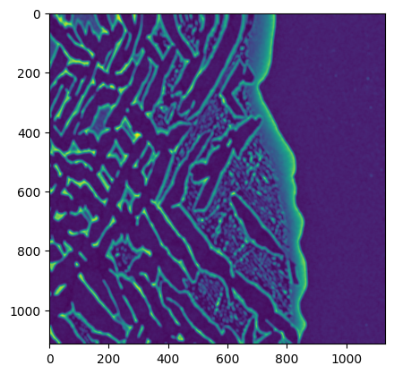
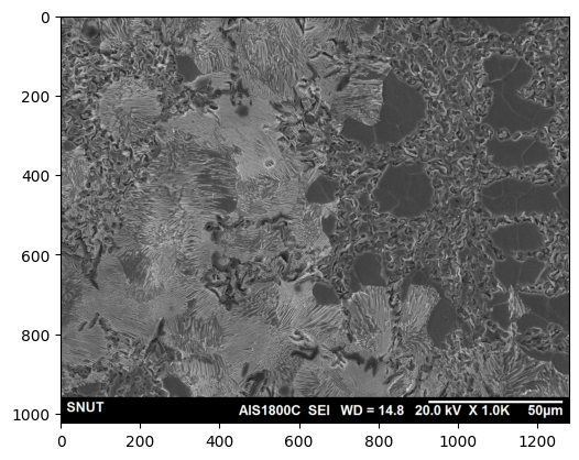
Image Data Format

Images serve as an important mode of representing scientific data, encompassing elements like metallographic micrographs, scanning electron microscope (SEM) images, and optical microscope imagery. Thankfully, Python offers a wide range of libraries that efficiently facilitate image reading. Specifically, in the original publications of this tool, a light micrograph panorama image was used to align results from electron back-scattered diffraction analysis and high-speed nano-indentation evaluations.

Most image formats can be handled by the cv2 or scikit-image libraries.

import skimage

limi_sk = skimage.io.imread("./data/example_image.jpg")
plt.imshow(limi_sk)

<matplotlib.image.AxesImage at 0x7fcd00813650>

You can use PIL also.

from PIL import Image

limi_pil = Image.open("./data/example_image.jpg")

By using strategies that we’ve visited above, you should be able to read most of scientific data.